Mixed Effects vs Fixed Effects Models

Mixed effects models (also known as multilevel models, hierarchical models, or mixed models) are statistical models that incorporate both fixed effects and random effects. They are specifically designed to handle data where observations are not independent, but rather clustered, nested, or hierarchical.

If running a standard Ordinary Least Squares (OLS) regression, a core assumption is that all data points are independent. However, in real-world data, this is often violated. Mixed effects models allow us to control for that non-independence without throwing away valuable variance.

Fixed Effects vs. Random Effects

To understand mixed models, it helps to break down the two components:

Fixed Effects: These are the variables we are primarily interested in analyzing. They represent population-level effects that are assumed to be constant (fixed) across all groups. For example, if we are analyzing the impact of “hours studied” on “test score,” the “hours studied” coefficient is a fixed effect.
Random Effects: These represent categorical grouping variables that introduce non-independence into our data. We assume these groups are a random sample from a larger population of groups. Instead of estimating a specific coefficient for every single group, the model estimates the variance between the groups. For example, if students are nested within different “schools,” the “school” would be a random effect.

Why Not Just Use Standard Regression?

Let’s create a scenario where we are predicting test_score based on hours_studied. We have 200 students clustered across 10 different schools. Each school has its own baseline performance level.

import pandas as pd
import numpy as np
import statsmodels.formula.api as smf

# Generate synthetic data
np.random.seed(42)
n_schools = 10
students_per_school = 20

# Create groups (schools)
schools = np.repeat(np.arange(n_schools), students_per_school)

# School-specific baseline scores (Random Intercepts)
# Some schools inherently start with higher or lower averages
school_effects = np.random.normal(loc=50, scale=10, size=n_schools)
baselines = school_effects[schools]

# Hours studied (Fixed effect variable)
hours_studied = np.random.uniform(1, 10, size=n_schools * students_per_school)

# Test scores = baseline + (slope * hours) + noise
# True slope is 5.0
test_scores = baselines + (5.0 * hours_studied) + np.random.normal(0, 3, size=n_schools * students_per_school)

df = pd.DataFrame({
    'school': schools, 
    'hours_studied': hours_studied, 
    'test_score': test_scores
})

import pandas as pd
import numpy as np
import statsmodels.formula.api as smf

# Generate synthetic data
np.random.seed(42)
n_schools = 10
students_per_school = 20

# Create groups (schools)
schools = np.repeat(np.arange(n_schools), students_per_school)

# School-specific baseline scores (Random Intercepts)
# Some schools inherently start with higher or lower averages
school_effects = np.random.normal(loc=50, scale=10, size=n_schools)
baselines = school_effects[schools]

# Hours studied (Fixed effect variable)
hours_studied = np.random.uniform(1, 10, size=n_schools * students_per_school)

# Test scores = baseline + (slope * hours) + noise
# True slope is 5.0
test_scores = baselines + (5.0 * hours_studied) + np.random.normal(0, 3, size=n_schools * students_per_school)

df = pd.DataFrame({
    'school': schools, 
    'hours_studied': hours_studied, 
    'test_score': test_scores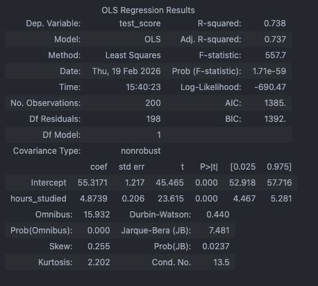
})

OLS Approach:

# OLS Model: test_score predicted by hours_studied
ols_model = smf.ols('test_score ~ hours_studied', data=df).fit()
print(ols_model.params)

# OLS Model: test_score predicted by hours_studied
ols_model = smf.ols('test_score ~ hours_studied', data=df).fit()
print(ols_model.params)

What happens here: The OLS model calculates a single intercept and a single slope for hours_studied. Because it ignores the massive variations between schools, the model’s standard errors will be artificially small, and the $R^2$ might be misleading. The model “thinks” it has 200 independent data points, but it really has 10 clusters of 20.

OLS: One Slope for Everyone

In a standard OLS regression predicting test scores from study hours across all schools:

${Score}_{i j} = β_{0} + β_{1} \cdot {StudyHours}_{i j} + ϵ_{i j}$

There is one global intercept $β_{0}$ and one global slope $β_{1}$ . Every school is assumed to have the same baseline score and the same relationship between study hours and performance. The model is blind to school structure entirely

Mixed Model Approach:

Now, we run a Linear Mixed Model (LMM). We specify hours_studied as our fixed effect, and tell the model to group the data by school as a random effect (specifically, a random intercept).

# Mixed Model: test_score predicted by hours_studied, grouped by school, Random Intercept 
mixed_model = smf.mixedlm('test_score ~ hours_studied', df, groups=df['school']).fit()
print(mixed_model.summary())

# Mixed Model: test_score predicted by hours_studied, grouped by school, Random Intercept 
mixed_model = smf.mixedlm('test_score ~ hours_studied', df, groups=df['school']).fit()
print(mixed_model.summary())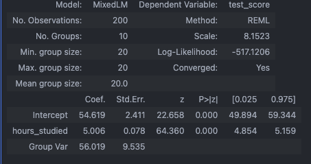

Mixed Model: Three Possible Configurations

Mixed models let you choose how much you allow schools to differ:

1. Random Intercept Only (Most Common)

${Score}_{i j} = (β_{0} + u_{0 j}) + β_{1} \cdot {StudyHours}_{i j} + ϵ_{i j}$

Each school gets its own intercept $β_{0} + u_{0 j}$ , but the slope is shared. This means study hours have the same effect in every school — but schools differ in their baseline performance. Lines are parallel but shifted up/down.

2. Random Slope Only (Rare)

Each school gets the same starting point but a different slope — meaning study hours help more in some schools than others, but baseline scores are identical. Unusual in practice.

3. Random Intercept + Random Slope (Most Flexible)

${Score}_{i j} = (β_{0} + u_{0 j}) + (β_{1} + u_{1 j}) \cdot {StudyHours}_{i j} + ϵ_{i j}$

Now each school has its own intercept AND its own slope. School A might have high baseline scores and a steep study-hours effect. School B might have low baseline scores but an even steeper effect. Lines are neither parallel nor anchored

# Random intercept + random slope
mixed_model = smf.mixedlm('test_score ~ hours_studied', df, groups=df['school'],re_formula="~hours_studied").fit()
print(mixed_model.summary())

# Random intercept + random slope
mixed_model = smf.mixedlm('test_score ~ hours_studied', df, groups=df['school'],re_formula="~hours_studied").fit()
print(mixed_model.summary())

In our example, Here is what that looks like for each config (except random slope):

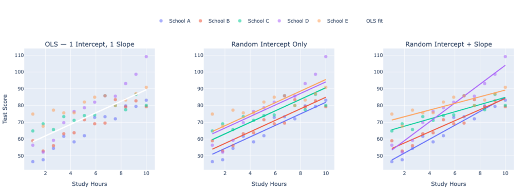
What Each Panel Shows

Panel 1 — OLS: All 5 schools’ student data is plotted, but a single white line fits everyone. It ignores the fact that schools have different baselines and different study-hour effects. The line is a compromise that fits no school particularly well.

Panel 2 — Random Intercept Only: Each school now gets its own colored line, but all lines are perfectly parallel — same slope, different vertical positions. The model acknowledges that School E starts higher than School A, but assumes study hours help equally in all schools.

Panel 3 — Random Intercept + Random Slope: Each school gets a line that is free to start anywhere and tilt at any angle. Some schools have steep slopes (study hours matter a lot), others are flat. This is the most realistic and flexible configuration

Visual Intuition

Model	Intercepts	Slopes	Lines look like…
OLS	One for all	One for all	Single line
RE: Random intercept	One per school	Shared	Parallel lines
RE: Random slope	Shared	One per school	Fan from one point
RE: Both random	One per school	One per school	Freely varying lines

Comparing the Outputs

When we look at the mixed_model.summary(), we will see a few distinct differences from standard OLS:

Fixed Effects Coefficients: We will still get a coefficient for Intercept and hours_studied. These represent the “population average” starting score and the “population average” effect of studying.
Random Effects Variance (Group Var): Instead of calculating 10 separate dummy variable intercepts for the 10 schools, the model outputs a Group Var (variance) metric. This number tells us how much the baseline test scores vary between the different schools.
More Accurate Standard Errors: Because the model correctly attributes a chunk of the variance to the school groups rather than lumping it all into the residual error, the standard errors and p-values for our fixed effects are mathematically sound and protect we from false positives.

What is the difference between anova and random effects model?

In a random effects model, the total variance in an outcome $y_{i j}$ yij (observation $j$ j in group $i$ i) is split into two components:

$Var (y_{i j}) = σ_{u}^{2} + σ_{ϵ}^{2}$

$σ_{u}^{2}$ = between-group variance (how much group means differ from the overall mean)
$σ_{ϵ}^{2}$ = within-group variance (how much individuals differ within their group)

The model explicitly estimates both. The ratio $σ_{u}^{2} / (σ_{u}^{2} + σ_{ϵ}^{2})$ is called the intraclass correlation (ICC) — it tells us how much of the total variance is explained by group membership.

So What Does ANOVA Do?

One-way ANOVA also partitions total variance into between-group (SSB) and within-group (SSW) components — and tests whether group means differ significantly. On the surface, this sounds identical. But the goals and mechanics diverge significantly:

Feature	One-Way ANOVA	Random Effects Model
Goal	Test if group means differ (hypothesis test)	Estimate the magnitude of group-level variance as a parameter
Group treatment	Groups are fixed, specific categories	Groups are random draws from a population
Predictors	Only group membership	Can include continuous covariates + group effects simultaneously
Output	F-statistic, p-value	Variance components $σ_{u}^{2}$ , $σ_{ϵ}^{2}$ , ICC
Repeated measures over time	Not naturally handled	Core use case (longitudinal/panel data)
Generalizability	Only to observed groups	To the broader population of groups

The Key Conceptual Difference

ANOVA asks: “Are these specific group means statistically different?” — it treats groups as fixed labels.

A random effects model asks: “How much does being in a randomly assigned group explain variation in the outcome?” — it treats groups as a source of structured randomness to be quantified and modeled, not just tested.

Example

Say we measure employee productivity across 20 companies.

ANOVA tests: “Are these 20 companies’ mean productivities significantly different?” It gives us an F-test. We can’t say anything about companies we didn’t observe.
Random Effects estimates: “How much of the variation in productivity is attributable to company-level factors vs. individual-level factors?” It gives we $σ_{u}^{2}$ and $σ_{ϵ}^{2}$ . If ICC = 0.4, then 40% of the variance is between companies. Crucially, we can also add a predictor like work-from-home policy alongside the random company effect — ANOVA can’t do this naturally.

Where They Overlap

Historically, variance components in random effects models were estimated using ANOVA-style sum-of-squares — this is literally called the ANOVA estimator for variance components. Modern software uses REML (Restricted Maximum Likelihood) instead, which is more efficient, especially with unbalanced data. So ANOVA is more like a computational ancestor of random effects, not the same model.

In short: ANOVA is a special, simpler case focused on testing fixed group differences. Random effects models are a richer framework that models group-level variation as a probabilistic quantity, handles covariates, generalizes to unseen groups, and scales to complex longitudinal or hierarchical data.